Turing machines and the busy beavers

For years I have been an avid reader of the Science website Naukas. The website is a carrier for online science popularization in Spanish. If you speak the language and love Science, I greatly encourage you to add it to your bookmarks.
In particular, I am a big (BIG) fan of Francis’ blog as well as Daniel’s blog that are part of the Naukas family.
I must admit that they have been an inspiration for the creation of this micro-blog. So, when I came across the article “Carnaval de Matemáticas: La función castor afanoso cumple 60 años” (Villatorio 2022) and the R code snippet of a Turing Machine simulator and a Busy Beaver, I couldn’t help but put together this small post and explore how to represent the Busy Beaver output using R.
Turing Machines
The Wikipedia (Wikipedia contributors 2022b) provides an excellent overview about the Turing Machines.
While some details may vary depending on the definition, basically, a Turing machine is an abstract machine - or theoretical model - consisting of :
- An infinite tape divided into cells. Each cell contains a symbol from a finite alphabet.
- A head that can read (scan) the symbol on the tape under the head or write a new symbol. The head can shift one cell at a time to either (L)eft or (R)ight.
- A state register that stores the current state.
- A table of instructions (states).
A new state is derived from the combination of the symbol in the tape and the current state, the machine runs till it reaches the state “H” (Halt).
Busy Beaver
Francis’ article (Villatorio 2022) is about Tibor Radó who discovered the Busy Beaver functions, a type of Turing machines, in 1962 (Rado 1962) and provides a brief context on the topic as well as the main references.
Below I bring over a simple description from Wikipedia to share some context.
… the busy beaver game consists of designing a halting Turing machine with alphabet {0,1} which writes the most 1s on the tape, using only a given set of states. The rules for the 2-state game are as follows:
- the machine must have two states in addition to the halting state, and
- the tape initially contains 0s only.(Wikipedia contributors 2022a)
The website Turing Machine Visualization is of great assistance in visualising Turing machines. Among others you can simulate and visualise a 3-state and 4-state Busy Beaver.
Next I share the code taken from Francis’ article with some minor changes.
 1## Turing Machine Simulator in R
 2## Based on Francis', in turn, based on Nick Drozd's code
 3##
 4## This 4-state busy beaver was proven by Allen Brady in 1983.
 5##
 6turing.string = '1RB 1LB 1LA 0LC 1RH 1LD 1RD 0RA';
 7M = 24;
 8##
 9turing.vector = unlist(strsplit(turing.string,' '))
10turing.table = matrix(turing.vector,ncol=2,byrow=TRUE)
11colnames(turing.table)=c('0','1')
12rownames(turing.table)=toupper(letters[1:nrow(turing.table)])
13
14library(knitr)
15kable(t(turing.table), caption = 'Table of states (instructions) of 4-state 2-symbol Busy Beaver')| A | B | C | D | |
|---|---|---|---|---|
| 0 | 1RB | 1LA | 1RH | 1RD |
| 1 | 1LB | 0LC | 1LD | 0RA |
I have changed the code to generate a numeric matrix describing the tape for each step ,from top to bottom, untils the machine halts, the numbers in the matrix hold the following meanings:
- 0: symbol 0 in cell
- 1: symbo1 1 in cell
- 2: head on symbol 0 in cell
- 3: head on symbol 1 in cell
 1##
 2tape = rep(0,M);
 3pos = M/2;
 4state = 'A';
 5##
 6tape.print = tape;
 7tape.print[tape==0]=0;
 8tape.print[tape==1]=1;
 9tape.print = c(tape.print[1:(pos-1)],tape.print[pos] + 2 ,tape.print[(pos+1):M]);
10##
11tape.matrix = matrix(tape.print,nrow=1);
12library(stringr)
13while (state != 'H') # H represents the Halt state
14{
15  SMS = turing.table[state, as.character(tape[pos])]; ## Symbol-Movement-State
16  tape[pos] = as.integer(substr(SMS,1,1));            ## write symbol in tape
17  pos = pos + switch(1+(substr(SMS,2,2)=='R'),-1,+1); ## move Right or Left
18  state = substr(SMS,3,3);
19  tape.print = tape;
20  tape.print[tape==0]=0;
21  tape.print[tape==1]=1;
22  tape.print = c(tape.print[1:(pos-1)],tape.print[pos] + 2 ,tape.print[(pos+1):M]);
23  tape.matrix = rbind(tape.matrix,tape.print)
24}Goal
Francis in his article raised a request for finding a better representation of the output of the 4-state 2-symbol Busy Beaver function.
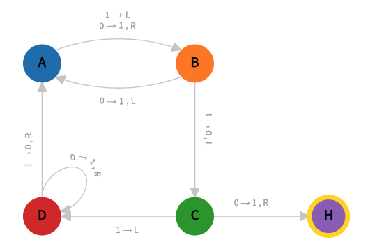
In Wikipedia one comes across the following representation of a 3-state Busy Beaver (Commons 2021):

This figure is used as a model for the the representations in this post.
Using plot.matrix
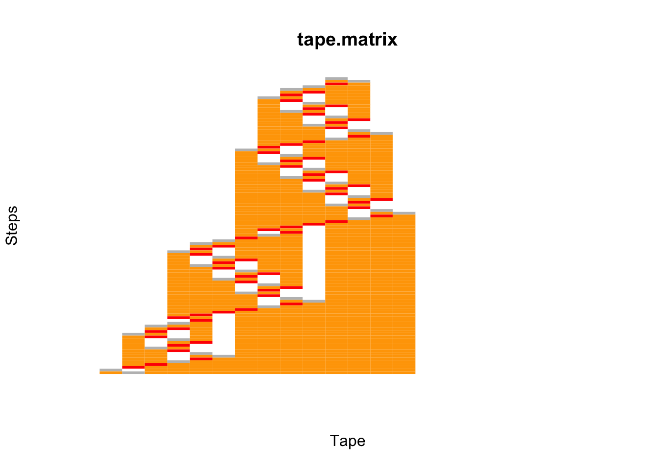
Below represents the very first attempt using the library plot.matrix.
1#install.packages('plot.matrix')
2library('plot.matrix' )
3plot(tape.matrix ,col = c('white','orange','grey','red'), key=NULL,axis.col = NULL,  axis.row= NULL, xlab='Tape', ylab='Steps', border=NA,polygon.cell = NULL)
This has been very easy, however I have found it difficult to apply further changes.
Using plotly
The second and most successful attempt so far is using plotly (Sievert 2020).
The challenge is getting a discrete colorbar so that one discrete colour is assign to the possible cell values. The article shares the trick to get this precisely.
 1library(plotly)
 2library(dplyr)
 3
 4colorScale <- data.frame(z=c(0,0.25,
 5                             0.25,0.5,
 6                             0.5,0.75,
 7                             0.75,1
 8               ),col=c('white','white','orange','orange','gray','gray','red','red'))
 9colorScale$col <- as.character(colorScale$col)
10
11fig <- plot_ly(z = tape.matrix,
12               type = 'heatmap',
13               ygap=1,
14               xgap=1,
15               colorscale=colorScale ,
16               width=300, height=600)
17
18fig <- fig  %>%
19  config(displayModeBar = FALSE, scrollZoom = FALSE) %>%
20  layout(plot_bgcolor='rgb(0,0,0)',
21             autosize = F,
22             xaxis = list(
23               constrain='domain',
24               title='Tape',
25               ticks = '',
26               tickvals = '',
27               range=c(0,M -1)
28               ),
29             yaxis = list(
30               title='Step',
31               autorange = 'reversed',
32               scaleanchor = 'x',
33               scaleratio = 0.8,
34               tickmode = 'linear',
35               dtick = 1,
36               tickfont = list(size=8)
37               ),
38             showlegend = F) %>%
39  colorbar(title = 'Tape cell',
40           len=0.2,
41           dtick =1,
42           tickvals=c(0.5,1.25,2,2.75),
43           ticktext=c(' 0 ',' 1 ','[0]','[1]'))
44
45figSo far, this approach has taken me closer to what I had in mind and within reasonable time. It hasn´t been easy or quick but I found the details I needed to move on.
Using ggplot2
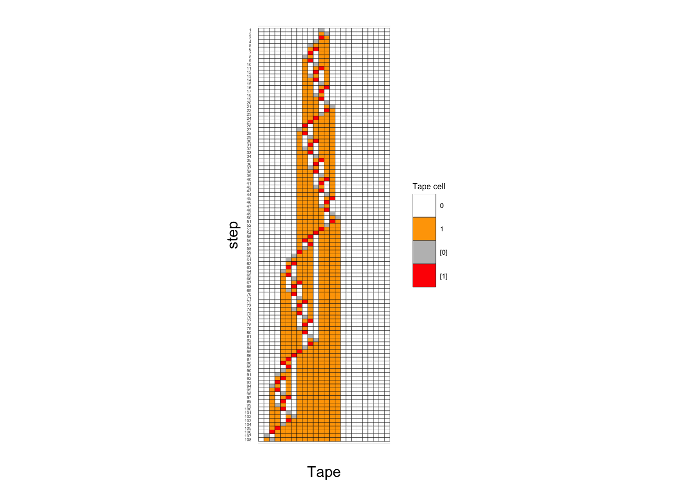
And finally, ggplot2(Wickham 2016).
 1library(dplyr)
 2library(reshape2)
 3df <- as_data_frame(tape.matrix)
 4df <- df %>% mutate(step = as.integer(rownames(df)))
 5df1 <- melt(df, id.vars = 'step')
 6df1<- df1 %>% mutate(value = factor(value))
 7
 8fig3 <- ggplot(df1, aes(x = variable, y = step))  +
 9  geom_tile(aes(fill = value),colour = 'black') +
10  scale_y_reverse(breaks=seq(nrow(tape.matrix) - 1,0,-1)) +
11  coord_fixed(ratio=0.7) +
12  xlab('Tape') +
13  theme_minimal() +
14  theme(axis.text.x=element_blank(),axis.ticks.x=element_blank(), axis.text = element_text(size = 3),legend.text = element_text(size = 5),legend.title = element_text(size = 6)) +
15  scale_x_discrete(breaks=NULL) +
16  scale_fill_manual(values=c('white','orange','grey','red'),name = 'Tape cell', labels = c('0', '1', '[0]','[1]'))
17fig3
With ggplot2 it took more less the same time to plot as plotly, however bear in mind that both do not deliver the same type of visulation. Preparing the data took definately longer.